COLLECTIVE BARGAINING AND TRADE UNION
Collective bargaining refers to the negotiations between a trade union and employer or an employer’s organization over the wages and work condition.
Trade unions.
Is the continuous association of wage earners for the purpose of monetary and improve paying of the workers and condition of working.
Example; in Tanzania we have TFTU –Tanzania Federation Trade Union.
FUNCTIONS OF TRADE UNIONS
- Bargaining on behalf of the workers for maintenance of better pay and good working condition i.e. provision of education, holiday recreations and
- To safe guard jobs. One should actual be sure of not losing job.
- To offer monetary benefits i.e. sickness and accident person.
- To restrict the supply of labour so as to maintain their demand i.e. the higher the demand, the higher wage rate.
- To keep all its members employed.
- To participate in national and international social economic organizations. E.g. ILO.
edu.uptymez.com
FACTOR AFFECTING THE STRENGTH / POWER OF TRADE UNION
-
The size of its membership.
If the trade union has large size of members, its strength will be large, likewise if the trade union shows a small size of its member its strength will be less.
- The extent of the effect it cause to the community or society to strike.
- General economic conditions of the trade unions.
- The nature of demand and supply of labour and product.
- Proportion of the wage to the total cost of production.
edu.uptymez.com
RENT (THE REWARD TO LAND)
Is the reward to the use of services of land, according to Ricardo.
Rent
Is that portion of produce of the earth which is paid to the landlord for the use of original and indestructible power of the soil.
How does rent arise
-
According to Ricardo opinion rent arise only on land not on other factors of production.
Because of the following peculiarities of land which are not found in other factors of production.
edu.uptymez.com
- Land is free. It is a gift of nature hence it has no cost of production from societies’ point of view.
- The supply of land is fixed and inelastic in the long run.
edu.uptymez.com
-
According to Ricardo “the continuous rise in population of the law of diminishing returns are the two principle reasons for the emergence of economic rent.
Thus According to Ricardo rent a rises because different plots of land have different fertility power.
Thus the difference in fertility power has been the reason for the emergence of economic rent.
edu.uptymez.com
What is economic rent?
Refers to the payment received by a factor over and above what is necessary to induce that factor to enter its present employment or to keep it there.
Transfer earnings
Refers to the minimum earning that must be paid to a unit of any factor to hold its present use. It is minimum payment that keeps a factor in the present occupation.
E.g. Economic rent = present earning – transfer earning.
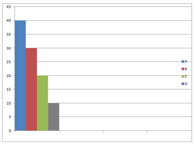
Consider rent under extensive cultivation.
| Grand of land | Total production in (000) | Rent (Tsh) |
| A | 40 | 40-10=30 |
| B | 30 | 30-10=20 |
| C | 20 | 20-10=10 |
| D | 10 | 10-10=0 |
edu.uptymez.com
Therefore, According to Ricardian theory rent can be measured as
Rent = output of extra marginal land – output of the marginal land
This also can be illustrated by using the graph below
Main conclusions of the Ricardian theory.
- Land is the only factor which posse’s original and indestructible power gifted by nature and those is the power which give rise to rent.
- Rent has a differential surplus since it arises due to differences in fertility and situation.
- To Ricardo rent was the result regardless of nature.
- As the price of corn is equal to the cost of production over the marginal or no rent land does not enter price. In other words the price of corn really determines land rent rather than having land rent determine the price of corn. On this basis Ricardo concluded corn is high not because of rent is paid but rent is paid because corn is high,
edu.uptymez.com
CRITICISM OF THE RICARDIAN THEORY
- He restricted rent to the land only while it is applicable to other factors of production. Rent is not the part of price of land. But according to modern economists rent does affect price.
- He implied that there will be no unit in all land if were fertile. Since rent is not only restricted to the fertility and but also infertility land.
-
He ignored the possibility that there were alternative uses of the price of land .This basically based on natural productivity land.
Even infertile land can be made fertile through reclamation process.
edu.uptymez.com
MODERN THEORY OF RENT
According to the modern theory developed by this Joan Robinson and others rent can rise on any factor of production. i.e land,capital, labour and entrepreneurship.
- According to the modern economist every factor has level element in other words. The supply of the factors of production is not perfectly elastic and hence they earn surplus income which is of the nature of rent.
- According to Mrs. Joan Robinson, the essence of the concept of rent is conception of surplus earned by a particular part of factor of production over and the minimum necessary to include it to do its work.
-
According to prof. Lip say, Economic rent is an excess over transfer earnings that a unit of the factors actually earns.
In short Economic rent = factors actual earnings – transfer earnings
That is; Economic Rent = present earning – Transfer earning
edu.uptymez.com
DETERMINATION OF ECONOMIC RENT
According to economic to modern theory economic rent arise due to scarcity and specificity of the factors of production.
Example
Suppose a mechanical engineers according in Kahama gold mining get $2500 as monthly pay. If he leaves Kahama Gold mining he can get $2000. In this situation $2500 is actually earning and $2000 is his transfer earnings that is the earning of the next best job.
This Economic rent = present earning – Transfer earning
= $us 2500 – $us 2000
= $500.
In other word the rent of to any factors of production will depend on its elasticity of surplus as follows;-
-
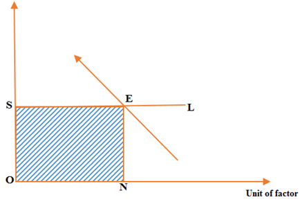
If the factors is perfectly elastic, supply will earn no rent because both its actual earning and transfer earning are equal
GRAPH
edu.uptymez.com
-
Present earning = SENO
Transfer earning = SEON
Rent =0
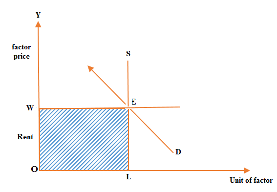
2. Rent under perfect inelastic. When the factor is completely specific or has only one specific use, change in price has no effect on its supply i.e even at zero prices the supply of the factor will remain the same.
Thus this factor has no transfer earning. Therefore the whole actual earning is the economic rent.
This is illustrated under the diagram below
edu.uptymez.com
From the diagram
Transfer earning = o
Present earning = WELO
Rent = actual earning – transfer earning
WELO – 0
-
Actual earning = Rent
3. Rent under relatively elastic supply.
It suggested that normally the supply of factors tend to increase with the increase in the factor price.
Thus the supply of the factor remain upward sloping comes from left to the right.
If the supply curve slope upwards all units to the left for the one being considered have lower transfer earning. Thus the total transfer earning of the units is the area below the supply curve. And the total payment (present earning) is equal to the total area.
edu.uptymez.com
This illustrated diagram below
From the diagram we note that;
Rent = present earning – transfer earning
RENO
– SENO = Res
Rent = RES
Thus the above analysis makes it clear that the more elastic the supply curve the less.
QUASI – RENT
The concept of quasi –rent was propounded and popularized by Prof. Marshall.
He used to explain the return of man- made produce goods the supply of which is fixed in the short period.
PRODUCTION FUNCTION
In a technical expression that indicates the relationship between output and the factor inputs used to produce such output.
In short production function can be written as;
Qx = f (K, L, E etc)
This can be simplified;
Qx = f ( k,l ) while l is variable and k is fixed.
TYPES OF PRODUCTION FUNCTION
-
Short run production function. Some factors are fixed while other are variable ie K (capital) is fixed labour is variable.
Qy = f(k,l)
It is subjected to the law of the diminishing returns.
-
Long run production function.
All the factors of production are variable. It is subjected to the law of return to scale.
edu.uptymez.com
| Land | Labour | Total output |
| 1 | 0 | 0 |
| 1 | 1 | 16 |
| 1 | 2 | 48 |
| 1 | 3 | 108 |
| 1 | 4 | 164 |
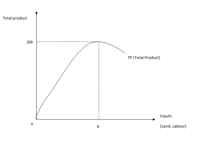
| 1 | 5 | 194 |
| 1 | 6 | 200 |
| 1 | 7 | 180 |
| 1 | 8 | 150 |
edu.uptymez.com
FACTORS DETERMINING THE PRODUCTION FUNCTION
- Quality of resources available.
- State of technology.
- Size of a firm.
- Price of factors of production.
- Political stability.
- Infrastructural facilities.
- Political making a factor.
edu.uptymez.com
TOTAL PRODUCT, AVERAGE PRODUCT AND MARGINAL PRODUCT
TOTAL PRODUCT :- Is the level of output which can be produced by a given amount of input.
Total product
= Labor
x Average product
Where L is labour.
AVERAGE PRODUCT AP
Is the output per unit of variable factors
AP = TP/L
Where by TP=Total Product
L=Labour quantity
Given
Q =2L2– L find average product.
AP=TP/L
AP=(2L2-L)/L
Divide L from the TP given.
Average product = 2L – 1
MARGINAL PRODUCT ( MP )
Is the addition to the total product that result to unit factor inputs.
Is a changes of total output as a result of unit change of a factor inputs.
MP=∆TP/∆L
Where by ΔTP=Change of total product
ΔL=Change of labour
TP=Total product
OR

Example:
Find marginal product of the following economics equation
Q=2L2-L
MP=SL/SQ
=TP/L
MP=2X2L2-1-1XL1-1
MP=4L-1
Assignment
The following table is demand from a production firm y.
| L | TP | MP | AP |
| 1 | 3 | 3 | 3 |
| 2 | 8 | 5 | 4 |
| 3 | 15 | 7 | 5 |
| 4 | 20 | 5 | 5 |
| 5 | 24 | 4 | 4.8 |
| 6 | 26 | 2 | 4.3 |
| 7 | 26 | 0 | 3.7 |
| 8 | 24 | -2 | 3 |
| 9 | 23 | -1 | 2.5 |
| 10 | 20 | -3 | 2 |
edu.uptymez.com
THE GRAPH MP, TP, AP
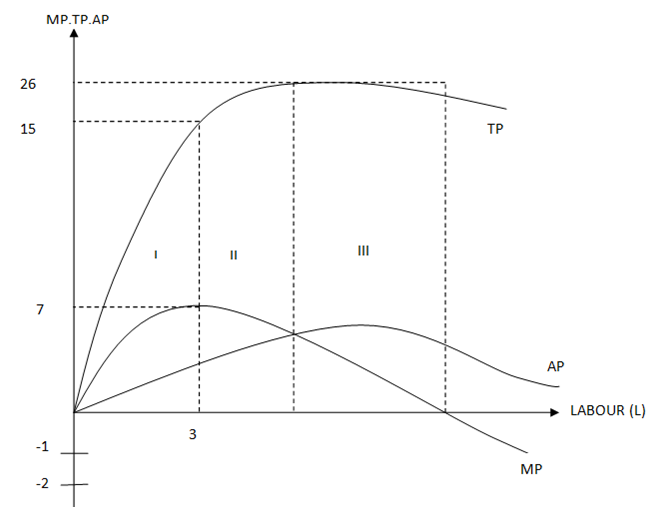
MP-Marginal Product
TP-Total Product
AP-Avarage Product
L-Labour Quality
G-Point of a Diminishing Returns.When quality labour employed are 3and marginal product rising up to and start to diminish.Total product increases from1 to 10. Average product increase until 5men are employed,then it deminish
The Law of Variable Proportions which is the new name of the famous Law of Diminishing Returns.
→According to Stigler” “As equal increments of one input are added, the inputs of other productive services being held constant, beyond a certain point, the resulting increments of produce will decrease i.e., the marginal product will diminish”.
→According to Paul Samulson “An increase in some inputs relative to other fixed inputs will in a given state of technology cause output to increase, but after a point, the extra output resulting from the same addition of extra inputs will become less”.
The law of variable proportions states that as the quantity of one factor is increased, keeping the other factors fixed, the marginal product of that factor will eventually decline. This means that upto the use of a certain amount of variable factor, marginal product of the factor may increase and after a certain stage it starts diminishing. When the variable factor becomes relatively abundant, the marginal product may become negative.
OR
Law of Variable Proportions:
“in a given state of technology, when the units of variable factor of production (L) are increased within the units of other fixed factors, the marginal productivity increases at increasing rate up to a point, after this point. it will become less and less”
Assumptions:
The assumptions of the law of variable proportion are given as below:
- It is assumed that the technique of production should remain constant during production.
- It operates in the short-run because in the long run, fixed inputs become variable.
- Some inputs must be kept constant.
- The various factors are not to be used in rigidly fixed proportions but the law is based upon the possibility of varying proportions. It is also called the law of proportionality.
- It is assumed that all the units of variable factors of production are homogeneous in amount and quality.
- It is assumed that labor is a single variable factor.
edu.uptymez.com
Schedule:
The law of variable proportion is explained with the help of the following schedule:
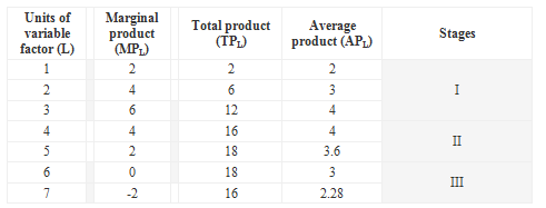
In the above schedule, units of variable factor (labor) are employed with other fixed factors of production. The marginal productivity of labor goes on increasing up to the 3rd worker. This is so because the proportion of workers to other fixed factors was at first insufficient. After 3rd worker the marginal productivity goes on falling onwards till it drops down to zero at the 6th unit of labor. The 7th worker is only a cause of obstruction to the others and is responsible in making the marginal productivity negative. The marginal productivity (MPL) and the average productivity (APL) equalize at 4the worker. Then the MPL falls more sharply
Diagram:
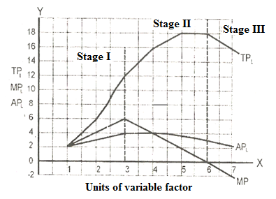
The number of workers are measured on X-axis while TPL, APL and MPL on Y-axis. The above diagram shows the three stages also obtained from the schedule.
Stage I:
At this stage MPL increases up to 3rd worker and its curve is higher than the average product, so that total product is increasing at increasing rate.
Stage II:
At this stage, MPL decreases up to 6th unit of labor where MPL curve intersects the X-axis. At 4the unit of labor MPL = APL after this, MPL curve is lower than the APL. TPL increases at decreasing rate.
Stage III:
At 6the unit of labor the MPL becomes negative, the APL continues falling but remains positive. After the 6th unit, TPL declines with the employment of more units of variable factor (L).
Relationship Among Total, Average and Marginal Product:
The relationship among total, average and marginal product of labor in the light of the law of variable proportion is explained as under:
- The marginal productivity of labor increases, the TPL also increases at increasing rate. It is shown in the schedule up till 3rd unit of labor. The MPL curve has positive slope and TPL curve has rising tendency towards Y-axis.
- When the MPL decreases onwards till it drops to zero, the TPL increases at decreasing rate as shown in the stage II and the TPL curve has positive slope but has rising tendency towards X-axis
- When the MPL is equal to zero, the TPL is maximum as shown on the 6th unit of labor.
- When the MPL becomes negative, the MPL curves falls below the X-axis, the TPL declines from its maximum position and its slope becomes negative as shown in the stage III in the above diagram.
- When the MPL increases, The APL also increases but at slow rate. The MPL curve becomes above the APL curve. Both have positive slopes.
- At some point, MPL = APL. At this point, MPL curve intersects the APL curve as shown at the 4th unit of labor in the above diagram.
- After intersecting point, MPL falls sharply. The MPL curve becomes below the APL curve. Both curves have negative slope.
- When MPL becomes negative, the APL never becomes negative because it is calculated from the TPL. So MPL curve is below the X-axis but APL curve is above the X-axis, having negative slope.
edu.uptymez.com
CAUSES FOR OPERATION OF THE LAW
- Fixed of a factor.
- Scarcity of a factor.
- Existence of imperfect substitutes. There is no way capital can be substituted to labour.
- Optimum combination of the inputs.
edu.uptymez.com
LIMITATIONS OF LAW OF VARIABLE PROPORTIONAL
(DIMINISHING RETURNS)
- Operates only in the short run.
- It is restricted to land only yet in reality it can apply to other factors when they are fixed.
- It is not applicable in case of virgin land because the land becomes productive for a long period.
- Variable factors are not homogeneous, that is they differ in efficiency ability.
- It does not consider the influence of other factors such as health of a worker.
edu.uptymez.com
Thus the operation of law of returns to scale is mainly caused by two major means,which are;-economics of scale and diseconomics of scale.
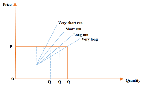
-
Very short run.
Refers to the period of time which is very short to make all factors variable i.e. that is all factor are fixed.
-
Short run.
Refers to the period of time where at least one factor is fixed and the other is variable.
-
Long run.
Refers to the period of time that is long enough to make all factors variable.
-
Very long run.
Refer to the period of time which is able to not only change factors of production but also the technology.
GRAPH
edu.uptymez.com
The law of return to scale of low production operates in long run while the law of Diminishing returns operates in the short run production function.
ASSIGNMENTS
Consider the following table and then answer the question that follows;
| Labor (L) | TP | AP | MP |
| 1 | 4 | 4 | 4 |
| 2 | 14 | 7 | 10 |
| 3 | 27 | 9 | 13 |
| 4 | 40 | 10 | 13 |
| 5 | 60 | 12 | 20 |
| 6 | 72 | 12 | 12 |
| 7 | 77 | 11 | 5 |
| 8 | 80 | 10 | 3 |
| 9 | 80 | 9 | 0 |
| 10 | 75 | 7 | -5 |
edu.uptymez.com
- From the table draw the curve to depict the law of variable proportion.
- Identify the number of labour at
- MP=AP
- Max=TP
- MP=0
edu.uptymez.com
SOLUTION
-
MP=AP
The number of labour at MP=AP from the graph is 6
-
Max = TP
The number of labour of maximum is 9
-
MP = 0
The point at that level MP = 0 is 9. Because the maximum is 9.
Given the following TP =2L2-20L
- Find the unit of labour which will maximize output.
- Calculate the TP, MP, and AP.
edu.uptymez.com
SOLUTION
From TP = 2L2-20L
= 2 x 2L(2-1)-20L(1-1)
= 4L – 20
The about at maxim MP = 0
MP = TP
0=4L–20
20/20=4L/4
5 = L
The unit of labour which will maximize the output is 5
MP, TP, and AP
TP=2L2-20L
TP =2L2-2L
AP = TP/L
= 2L2-20L
= L(2L-20)/L
= 2L – 20
= (2(25)-20(5))/5
= -50/5
AP= -10
The average product can’t be -10 is +10
TP = 2(25) – 20(5)
= 50 – 100
= -50
The product can’t be negative then ignore negative and therefore TP = +50
TP =2L2-20L
= 2(25) – 20(5)
= 50 – 100
= -50
The product can’t be negative then ignore negative and therefore TP = +50
MP = ∆TP/∆L
MP = 2L2-20L
= 2(2L)(2-1)-20L(1-1)
= 4L – 20L
= 4L -20
Where L= 5
MP = 4L – 20
= 4(5) – 20
= 20 -20
MP= 0
The marginal product is 0