- Creating a simple worksheet
edu.uptymez.com
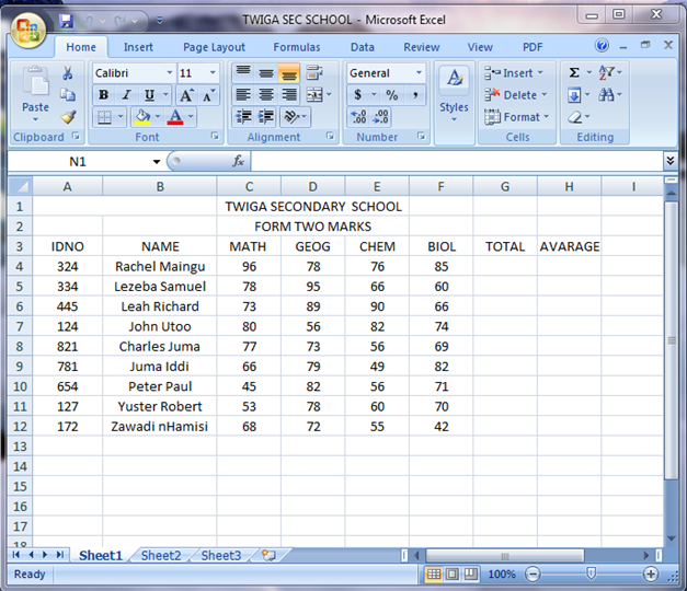
Instructions are given for creating the worksheet shown below. The first stage is to get the correct values in the cells. Later you can make the worksheet more attractive by the use of bold text, different alignment and color.
5.1. Entering the data
- Click in cell B2 and type
edu.uptymez.com
Twiga secondary school
- Press the Enter key (or one of the arrow key).
- Click in cell B4 and type
edu.uptymez.com
ID NO.
- Press the down-arrow key to move to cell B5
- Type
edu.uptymez.com
Rachel Maingu
- Press the down-arrow key and then complete column B as shown above.
- Enter the data in columns D, E, F and G (but not H and I)
edu.uptymez.com
5.2. Amending data
If you are in the process of entering data in a cell and you notice that you have made a mistake, it is easy to correct it. Press the Backspace ( ) key to delete a character to the left of the cursor or the Delete key to delete a character to the right of the cursor.
If you want to edit the contents of a cell you dealt with earlier, you should double-click in that cell and make the alternations either in the cell itself or on the formula bar.
If you want to clear a cell of its contents (formula and data), formats, comments or all three you can selects that cell with a single click of the left mouse button, select clear from the Edit menu and then click on contents F
formats,
Co comments, or All.
There are a couple of quick ways of clearing the contents of a cell. The first is to use the right mouse button to click in the cell and then select clear contents from the menu that appears. The second is to select the cell by clicking the left mouse button and the press the Delete key on the keyboard.
Do not confuse using the Delete key with selecting Delete from the Edit menu. That command carries out the more drastic action of removing the entire cell from the worksheet and shifting the surrounding cell to fill in the resulting space.
5.3. Ranges
In Excel, any rectangular area of cells is known as a range. The range is defined by the top-left and bottom –right corner cell references separated by a colon(:).
So, B4:D7 represents the range of cells cornered by B4 and D7.
5.4. Copying and pasting
The text in cell E5:E8 ( in other words E5, E6 and E8) is the same as in the range B5:B8 so you can copy that.
- Point to cell B5 and hold down the mouse button
- Keeping the button held down, drag the pointer to B8 and then release the mouse button. The range B5:B8 will be highlighted.
 Click on the copy button on the toolbar (or selected Copy from the Edit menu).
- Click in E5 (where you want the copy to be place).
 Click the Paste button on he toolbar (or select Paste from the Edit menu).
edu.uptymez.com
In addition, there is a smart tag(the Past Options one) near the bottom right-hand corner of the pasted data.
A smart tag can be:
- Ignored –it will disappear when you carry out some other action
- Removed –by pressing the Esc key
- Used – point to it and click on the down arrow to display several options; select one and press the Enter key
edu.uptymez.com
For now, just ignore the Paste Options smart tag and finish the process of entering the data.
- Click in any cell to remove the highlighting
- Press the Esc key to remove the flashing dotted line (marquee) round the cells you copied.
edu.uptymez.com
Note: selecting non-contiguous ranges
If you need to select cell that are not contiguous, (ie, ranges that are not necessarily next to each other), proceed as follows.
- Select the first area of cells
- Hold down the Ctrl key while selecting the other areas.
edu.uptymez.com
5.5. Adjusting the width of columns
If the Twiga secondary school text is too wide for columns B try widening those column.
- Move the cursor to the division between the areas containing the column names. Note how the shape of the cursor has changed to a vertical black line with arrows pointing right and left.
- Double –click the left mouse button.
edu.uptymez.com
The column will be widened (if necessary) automatically.
If you wish to have control over the sizing of the column, it can be done manually.
- Move the cursor to the division between the areas containing the column names
- Hold down the left-hand mouse button and drag that column divider the required distance to the right
- Release the mouse button.
- Repeat the process if you want to make fine adjustments.
edu.uptymez.com
5.6. Entering currency values
If you have column containing amounts of money. You do not have to type the ₤ sign, instead you can enter the numbers and format the cells as currency later.
Formatting the cells
- Highlight the cells ie F5 to F7 (Point to F5, press the mouse button; while keeping the button held down, drag the pointer to F7; release the button.)
- Point to the highlighted area and click the right mouse button.
- Choose Format Cells window, click on the Number tab (unless it is already selected.)
- In the Format cells window, click on the Number tab (unless it already selected).
- In the category: box select Currency by clicking on it.
- Make sure that Decimal places: is set to 2; symbol: show ₤ and that the first option in the Negative numbers: box is highlighted. Sample: shows you what the result of the formatting will be (₤0.50).
- Click on Ok.
edu.uptymez.com
Alternatively, you could have formatted the cell first and then entered the values.
If you begin a numerical entry with a ₤ sign, Excel assigns currency format to that cell. Similarly. If you end a numerical entry with a % sign, Excel assigns Percentage format to that cell.
Note: Excel 2003 includes the Euro symbol € for currency.
5.7. Formatting a cell before entering a value
Now try formatting a cell before entering its value.
- Click in F4

 Click on the Bold and Align Right buttons. The cell will not look any different until you enter a value
- Type
edu.uptymez.com
Costs
And press the Enter key.
The text should be in a bold front and right-aligned in the cell.
5.8. Formatting text
You have entered all the data you need but you might like to make the worksheet easier to read by formatting some of the text.
First make the word Allocation bold.
- Click in B4.
 Click on the Bold button on the toolbar.
edu.uptymez.com
Next apply a bold font to Adult in C4 and child in D4 and center the text in the cells as follows:
- Highlight cells C4:D4
- On the toolbar, click on the Bold, italic and Center button. If you can’t remember which those are, try pointing to each button in turn –a small pointer message will appear showing its name.
edu.uptymez.com
Next apply a bold italic font to Adult in C4 and Child in D4 and center the text in the cells as follows
- Highlight cells C4:D4


 On the toolbar, click on the Bold, Italic and Center buttons. If you can’t remember which those are, try pointing to each button in turn
edu.uptymez.com
–a small pointer message will appear showing its name.
5.9. Using different sizes and colors
The charity Barbecue heading of this worksheet can be made more interesting by changing its size and colour.
- Click in B2.
- Click on the down-arrow of the Font Size button
- Select another size, for example, 12.
edu.uptymez.com
Your text in B2 will increase in size.
 Click on the down-arrow of the Font color button.
- Select a suitable colour for your text.
edu.uptymez.com
It is possible to colour the background of cells and to centre a heading across a range of cells.
- Highlight the cells B2:F2
 Click on the down-arrow of the Fill color button.
- Select a suitable colour for your background. Be sure to make it different from the colour of your text or you will not be able to see the heading!
- Make sure that the range B2:F2 is still selected and click on the Merge and center button. Your heading will be centered in that range of cells.
- Click in any cell away from the heading.
edu.uptymez.com
5.10 Naming a sheet
The information on sheet 1 might refer to Twiga Secondary School to be held in Term II. It would make sense to name the sheet accordingly.
- Right –click on the tab sheet 1
- Select Rename from the menu that appears
- Type
edu.uptymez.com
Term II
And press the Enter key (or click in a cell).