COMPUTER/ICT NOTES FORM TWO TOPIC:2 SPREAD SHEET

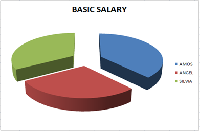
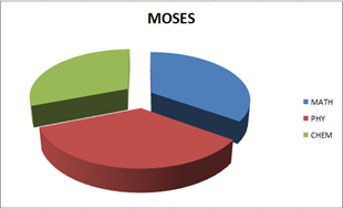
GRAPHS AND CHARTS

Data may be presented in graph or charts as well.

From the table below

To change the colour, click on the bar you want to change the colour.
If you want to change that chart type,click on the on the chart and insert,select the type of chart.

PAGE PROPERTIES AND PRINTING

Includes:-

1)      PAGE SETUP

It may include

a)      Header footer setup

b)      Selecting a printer

c)      Paper layout (page layout)

Procedures

From the menu bar, click file then select page set up.

        i.            Page tab

• On the page tab you may choose either portrait or landscape for the page layout.
• Select the page size as A4

edu.uptymez.com

      ii.            Header/footer

• Click header/footer tab
• Click custom header
• There are three sections here, you, may type your header in any section depending on what type of the paper do you want your footer/header to appear. But in most cases the left section is prefered for header.
• After typing your header click OK.
• Then click on custom footer.

edu.uptymez.com

The footer may be either in the center section or right section

• Click on the center section
• Click the button shown as # the word and page will disappear in the centre section also, data and time may be set in the footer right section. After completion of footer and header setup click OK>

edu.uptymez.com

PAGE PREVIEW.

From the Menu bar click File.

Then select print preview.

Note: Your page may default to two pages while the document is for one page only.

Procedures:

Click page break preview

Click OK to the window appearing.

If the document is making up two pages, there must be dotted separating those pages. Place your cursor on the dotted line and drug it to the right until you meet the solid line

WORKING WITH MS EXCEL WHILE YOU ARE IN MS WORK

Select ms excel form tools bar , work with your data

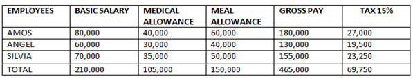
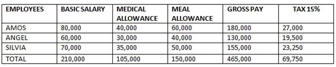
THE FOLLOWING IS SUMMARY OF PROCUREMENT

To shift/Return to Ms Excel Double click the Table.

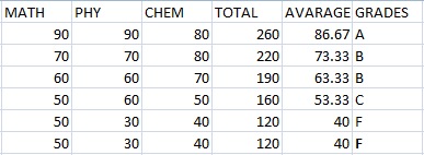
EXERCISE

From the given data below,

1. Find, total, Average, and Grades
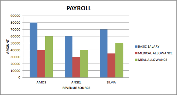
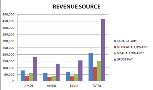
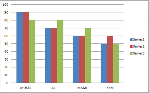
2. Draw bar graph, pie chart
3. Save file name with your name
4. Put the file in folder, save in desk top an my document

edu.uptymez.com

Formulating the formula

Note =, the number of opening brackets must be the same as closing brackets

Example, a student whose average is equal, or greater than 80, is placed in A grade, average equal or greater than 70 is grade B, average equal or greater than 50 is in C grade, otherwise F grade.

FORMULA

=IF(F2>=80,”A”,IF(F2>=60,”B”,IF(F2>=50,”C”,”F”)))

           

          

EXERCISE
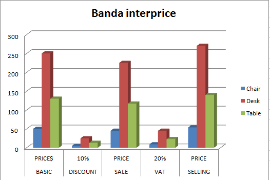
Banda Enterprises had the following data.

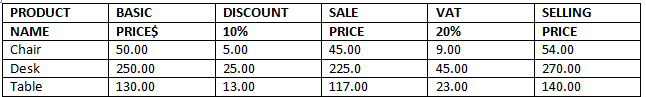
FORMULA:
Discount=Basic price * Discount
Basic Price
VAT=Sale Price* VAT
Selling price*VAT
Selling Price = Sale Price + VAT

Question

1.Present your information in Chart form (column chart)
2.Cut the graph and copy it on the separate worksheet and rename worksheet as chart
3.Create header and footer
4.”Excel test”as header (left section)
5.”You name,Data and time as footer(left section)
6.Save the work in your name and put it in the folder “on the desktop (My work)

1CHART
Answer 2